Practice note of presentation

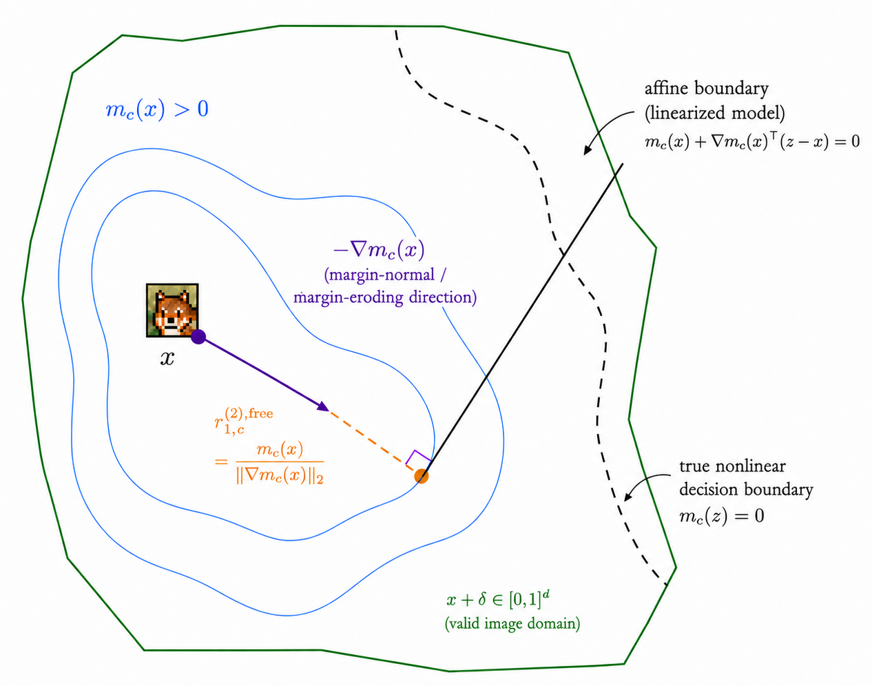
Slide 5: First Correction: Clean-Endpoint First Order

What do we actually mean by clean-endpoint first order? It is basically a one-point snapshot of the classifier.

We start from the clean image here, $x$ . At this point, the network tells us two things: how much class margin is left, $m_{c} (x)$ , and which local direction decreases that margin fastest, $- \nabla m_{c} (x)$ .

🌂 This purple arrow is that local margin-eroding direction. Importantly, at this stage we have not moved anywhere yet — all of this information is read at the clean point.

🏴 Now comes the ‘first-order’ step. We freeze this local slope. In other words, we pretend the margin continues to change exactly as it does right here. That turns the nonlinear problem into this simple affine boundary.

👑 Then we ask a very simple question: under that local linear model, how far would we have to move before the margin reaches zero? That distance is the first-order radius.

r_{FO} (x) = \frac{m_{c} (x)}{{‖ \nabla m_{c} (x) ‖}_{2}}

┉ Of course, the real network does not have to keep behaving this way. The true nonlinear boundary can bend away from the affine prediction. And that is exactly what the next part of the paper studies: what happens after we leave the clean point.

Slide 10: Why is s(t) the same at every cut?

Think of the network as one long chain. At any layer, I can cut that chain into two pieces. The first piece tells me what the original perturbation has become by this point. The second piece tells me how much a change at this point will still affect the final class margin. If I move the cut, both pieces change — but together they still represent the same original input-to-margin effect. So $s (t)$ cannot depend on where I choose to cut the network.

The decomposition changes. The end-to-end effect does not.

Think of the network as one long chain of multiplications. If the full chain is $2 \times 3 \times 4 \times 5 \times 6$ , I can cut it after 3, after 4, or after 5. The number on the left changes, and the number remaining on the right changes, but their product is still the same full chain.

(2 \cdot 3) (4 \cdot 5 \cdot 6) = (2 \times 3 \times 4) (5 \times 6) = 720

(👈)Pick any cut in the network. From the input up to this cut, we simply propagate the original route perturbation forward. Whatever that perturbation has become here, I call $z_{ℓ}$ .

(👉)Now look from the other end. Starting from the final class margin, ask how sensitive that margin is to motion at this same layer. That is $a_{ℓ}$ .

So at the cut we have exactly two pieces: what the perturbation has become, and how much that motion matters to the final task. Pairing them gives the same boundary-eroding sensitivity $s (t)$ .

“The cut only tells us where we choose to meet in the middle.”